Flow Matching

Introduction

Flow matching is a fundamental algorithm used in state-of-the-art image generation models as well as VLA (vision-language-action) models in robotics. In particular, $\pi_{0.5}$ (Physical Intelligence, 2025) and X-VLA (Zheng et. al., 2025) are notable high-performing examples of successful flow matching used in robotic manipulation.

I thought it would be interesting to dive into the mathematical derivations behind algorithm, standing on the shoulders of many excellent existing resources explaining it :)

What is Flow Matching?

The aim of flow matching is to generate a sample from an unknown probability distribution.

For example, let’s consider an image generation model. Say we have a dataset of 50 cat pictures and we want to generate another picture. The unknown probability distribution here is the mathematical function describing the likelihood of all cat pictures. We cannot know this function directly; we only have samples (our dataset). We want to sample from this unknown probability distribution to generate a picture that is distinct to the ones in the dataset, but one that we would still classify as a cat.

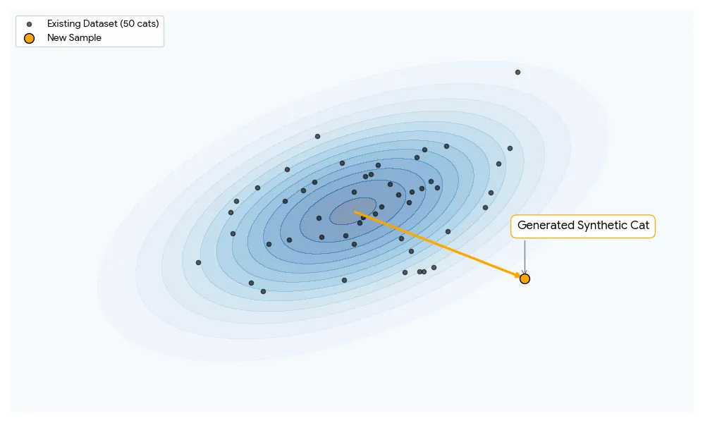
Blue represents the entire cat picture distribution, black dots represent our limited dataset.

How might we accomplish this? Flow matching proposes we build a path translating from a known distribution to this unknown distribution, so that if we follow this path, we will always end up at some point in the unknown distribution.

It’s sort of like a treasure map. It tells you where to go from where you started, and if you dig around the target, you’re bound to find treasure.

Let’s call the unknown target distribution $X_1$, and the known distribution $X_0$, where $X_0 = \mathcal{N}(0, I)$. Let’s set it such that at time $t=0$, $x \sim X_0$, at $t=1$, $x_1 = x \sim X_1$, so as we move forward in time we move closer and closer to the target distribution.

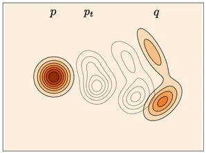
$p$ is known, $q$ is target, $p_t$ is our path (Lipman et. al., 2024)

Now let’s construct a probability path $p_t(x)$ that fulfills these requirements.

Constructing the Probability Path

At a given time $t$, $p_t(x)$ should give us the intermediate probability distribution (the grey distributions in the image above) that our points could possibly be in. By the marginal Law of Total Probability, given two continuous random variables $X$ and $Y$,

Thus, we can derive the probability path below! Given an arbitrary time $t \in [0, 1]$ and $q(x_1) = P(x_1)$,

As we can see, by defining $p_{t|1}(x|x_1)$ as a Gaussian with $\mu = tx_1$ and $\sigma = (1-t)I$, we can intuitively linearly interpolate over the variable $t$ from $X_0$ to $X_1$. This specific probability path is the conditional optimal-transport or linear path.

Let’s define $X_t$ as the random variable given time $t$ using the Reparameterization Trick.

Now we have $X_t$ in terms of $X_0$ and $X_1$.

Let’s take a step back and remind ourselves of the goal. Given a sample from a known probability distribution, we want to be able to map it to a sample from an unknown probability distribution. We now know how to describe a relationship between the probability distributions $X_0$ and $X_1$ by interpolating over intermediary probability distributions $X_t$, but $X_t$ is still incalculable without knowing what $X_1$ is.

Additionally, this is not the function input/output we want. We want to be able to map from an input, to some output when $t=1$.

Defining Flow and Vector Fields

This is where flow and vector fields come in.

Let’s define a vector field $u_t(x)$ such that given coordinate $x$ and time value $t$, $u_t$ outputs the direction to move from that point.

Let’s further define a flow $\phi_t(x_0)$ such that given a starting point $x_0 \sim X_0$ and $t \in [0, 1]$, it returns the coordinates of that point as we follow the vector field over time.

The relationship between the two can be defined as

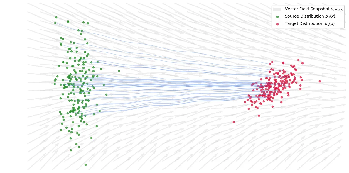
Arrows represent the vector field, the blue lines represent the flow given a starting input sampled from $x_0$

In the image above, we can see that as we move forward in time, we follow the vector field defined by the grey arrows, and our path that we’re creating is our flow!

For this vector field specifically, let’s define $u_t$ such that it creates the probability field $p_t$. This means that if we (hypothetically) sampled 1000 points from $X_0$, found their position at $t=0.5$ after following $u_t$, it would create the density represented by $X_{0.5}$.

This is an important enough concept to reiterate. A vector field dictates which way the point moves at a given time step. The flow represents the path a particle takes, given a starting location and what time step we’re at. The probability path represents the density of those particles.

(I’d recommend watching 3Blue1Brown’s video on this - his visualizations are extremely helpful)

Now we finally have the function we wanted! A vector field tells us how to move from a point in $X_0$ to a point in $X_1$. If we’re able to learn the correct vector field, we can generate any photo from our target distribution.

We can simply define the flow matching loss as

where $u_t^\theta$ is our neural network parameterized vector field. Minimizing this means our neural network perfectly matches the target vector field $u_t$.

Unfortunately, calculating this loss function is intractable.

Simplifying the Intractable Loss Function

Let’s first show why it’s intractable by deriving an equation for $u_t$.

You’ll notice that I began talking about particles rather than points: some students of physics may recognize this as fluid dynamics. Fluid dynamics theory further tells us that through the Continuity Equation,

where $\nabla \cdot (p_t u_t)$ is divergence, defined by

where x is a single point.

Multiplying $p_t(x)$ and $u_t(x)$ gives us the probability current (or flux), as $p_t(x)$ represents the density at a point and $u_t(x)$ represents the velocity of that point. Thinking about this in terms of liquids and a hose,

• low density and high velocity => medium amount of water coming out
• high density low velocity => medium amount of water coming out
• high density high velocity => high amount of water coming out

Flux represents how much water is flowing through a point at a given time.

Divergence defines how much a vector field is expanding / compressing at a specific point. Interpreting the continuity equation, if divergence is positive and the flux is expanding, then the change in probability (density) will be negative, meaning that more water is escaping. If divergence is negative and the flux is compressing, then the change in probability is positive, as the water is moving slower and thus more dense.

We can attempt to solve for $u_t(x)$ now. Starting with the Continuity Equation:

Substitute the marginal definition $p_t(x) = \int p_{t|1}(x|x_1)q(x_1)dx_1$ into the first term:

Move the time derivative inside the integral and substitute the conditional continuity equation $\frac{\partial p_{t|1}}{\partial t} = -\nabla \cdot (p_{t|1} u_{t|1})$:

Rearrange to equate the divergence terms:

Removing the divergence operator implies equality of the fields. Solving for $u_t(x)$ yields:

Unfortunately, we then find that $p(x_1|x)$ is intractable, as finding the integral over $x_1$ of this requires us to check every possible image to calculate it (and it’s impossible to check every single possible cat photo in existence).

Instead, we can simplify this by choosing a single objective, by fixing $x_1$ to be a single target example (i.e. an image in our dataset). Then we have an equation for $X_{t|1}$ which only depends on our Gaussian sample $X_0$ and $t$:

In this case, rearranging the identity $\frac{d}{dt}X_{t|1} = u_t(X_{t|1} | x_1)$ by differentiating Equation 14 yields

(Technically velocity fields should be a function of the current location not the target location, so you may rewrite this as $\frac{x_0-X_t}{1-t}$, but for our purposes they are equivalent.)

Finally! We have a much simpler velocity field function that we can now easily compute the MSE of, yielding the Conditional Flow Matching loss function.

At a high level, we are just stating to match a vector field that results in a linear path pointing from $X_0$ to $x_1$. Does this work? Finding the derivative of our earlier loss function $\mathcal{L}_{FM} \theta$ and this one will yield the same result, showing they are equivalent!

We can see this in example flow matching code (Lipman et. al., 2024):

import torch 
from torch import nn, Tensor

class Flow(nn.Module):
    """ 
    Parameterized vector field.
    Input: [x_t, t]
    Output: u(x_t)
    """
    ...

...

# Initialize flow matching model, MSE loss function
flow = Flow()
loss_fn = nn.MSELoss()

# x_1 sampled from target distribution, x_0 sampled from Gaussian 
# Calculate delta between the two
dx_t = x_1 - x_0  

# Find MSE between u^theta_t(x_t) and x_1 - x_0!
# Note that x_t represents the coordinates of the point while t is a float between [0, 1] representative of the time
loss_fn(flow(x_t, t), dx_t).backward()

I’ll leave the post there - maybe I’ll write more later on. Further reading would include various ODE solvers, score-based generative modeling, and diffusion models!

Resources that greatly helped me:

• https://ai.meta.com/research/publications/flow-matching-guide-and-code/
• https://diffusion.csail.mit.edu/2025/index.html